na

ESRI: SPATIAL ANALYST 

Module 1: Getting Started with Arc GIS Spatial Analyst; This module introduces the types of analysis I can perform using the ArcGIS Spatial Analyst extension. I learned what to keep in mind before undertaking an analysis and how to set up the analysis environments to control input and output datasets. I also learned how to convert between raster and vector data, as well as how to reclassify rasters.

^ (Framework_2) This exercise,  introduced me to several ways to run Spatial Analyst tools while setting the environments as well.

^ (Convert2) This exercise taught me to convert vector data to raster data. First I looked at the effects of setting an analysis extent, then I looked at the effects of setting an analysis mask.

^ (ReclassElev2) In this exercise, I reclassified an elevation raster into four general elevation zones. I also created the zones using two different classification methods so I can see how the map changes.

^ (ReclassRemap2)In this exercise, I reclassifed a raster using an ASCII remap file.

^ (ReclassVeg2) In this exercise I reclassified a vegetation raster based on sensitivity to drought. i then limited the results to the study area.

I am now able to:

• Understand how ArcGIS Spatial Analyst fits into the geoprocessing framework.
• Set up an analysis environment.
• Run Spatial Analyst operations using a tool dialog box, the command line, and a model.
• Convert between feature and raster data.
• Reclassify data.

Module 2:  Analyzing Surfaces; I learned how to derive new data from surfaces using the surface analysis tools: slope, aspect, and viewshed. Slope is a measure of the steepness of elevation change. Aspect is the compass direction of a slope. A viewshed is the visibility of surface areas from observation points.

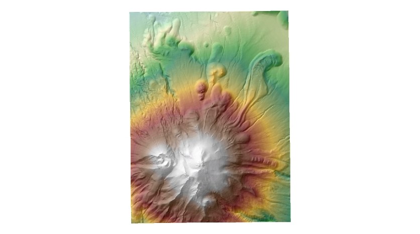
^  In this exercise (Hillshade2) I  created a hillshade from an elevation raster and displayed another layer over it.

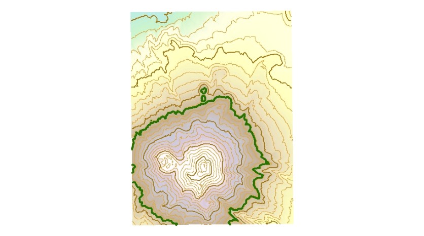
^ In this exercise (Contour2) I created contours from an elevation raster.
 

^ In this exercise (SlpAsp2) I computed both slope and aspect.  I also learned how to calculate slope and aspect using the Slope tool and the Aspect tool. Slope measures the incline, or steepness, of a surface and expressed  it in either degrees or percent slope.  
 

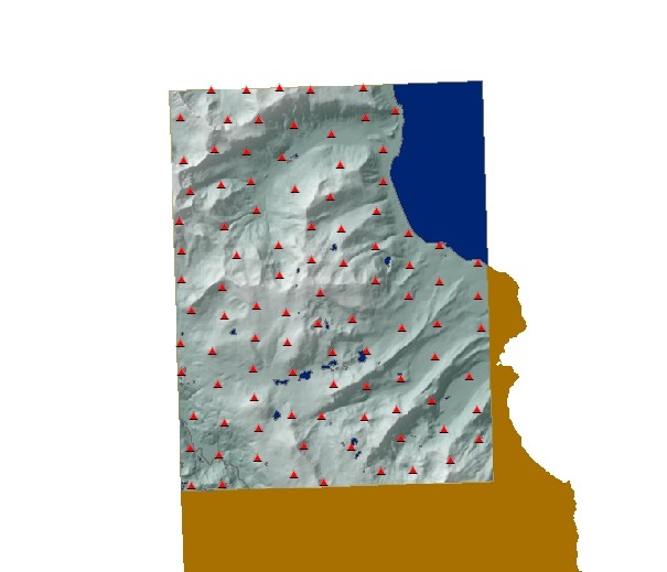
^ In this exercise (Viewshed2) I looked for areas suitable to locating a radio communications repeater tower. The new tower site must be able to "see" the existing towers within the study area.

 

I am now able to:

• Generate contours.
• Create hillshades.
• Calculate slope.
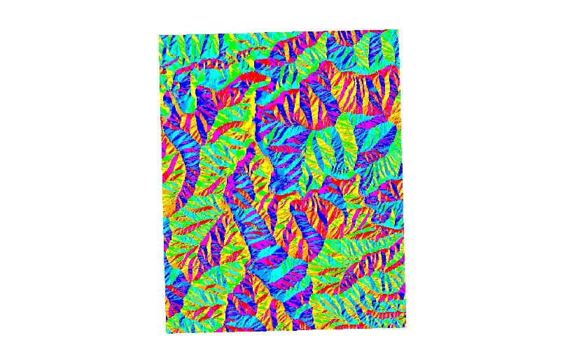
• Calculate aspect.
• Calculate viewshed.

 Module 3:  I learned how to use Map Algebra operators and functions to build my own expressions.  I also learned how to perform some of the most useful tasks in Map Algebra, such as conditional processing, testing for NoData, and setting cells to NoData.

^ (Functions2) My approach was to compute a hillshade for the middle of each month, placing the sun in its correct location, and deriving the average sun exposure for the six months.

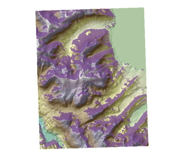
^ (Calculations2) In this exercise I combined Map Algebra operators and functions to model the best location to raise pine and fir trees to be used for reforestation. I know that these types of trees grow best above 2,400 meters elevation. Also, I have an agreement with the United States Forest Service that will allow me to develop the farm on their lands.

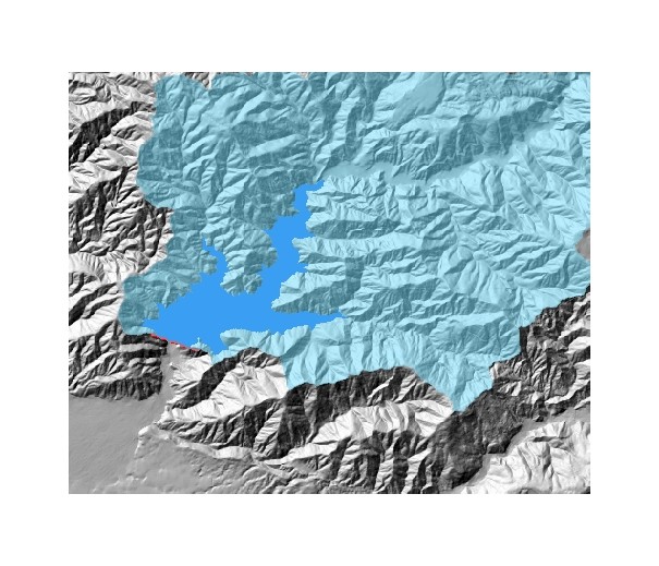
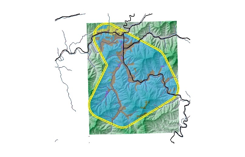
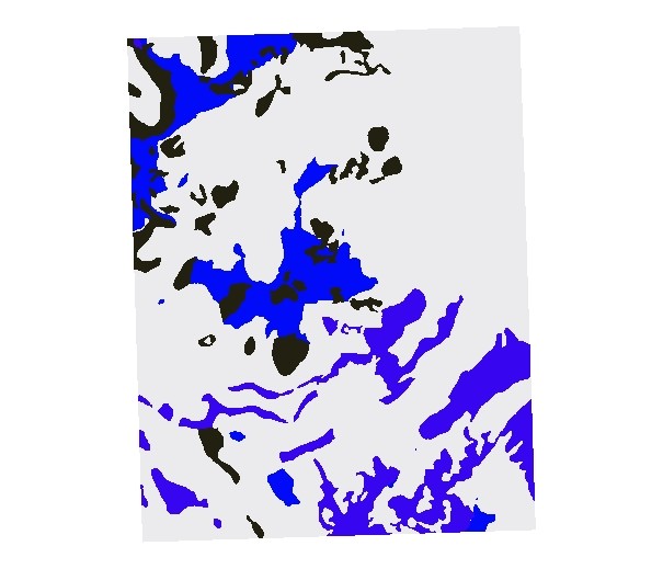
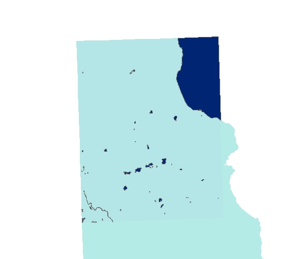
^ (Conditional2) In this exercise I used CON to find the potential reservoir created by a proposed dam within a basin. I found the reservoir, then used the CON function with the ISNULL function to update an elevation raster with the new water surface.

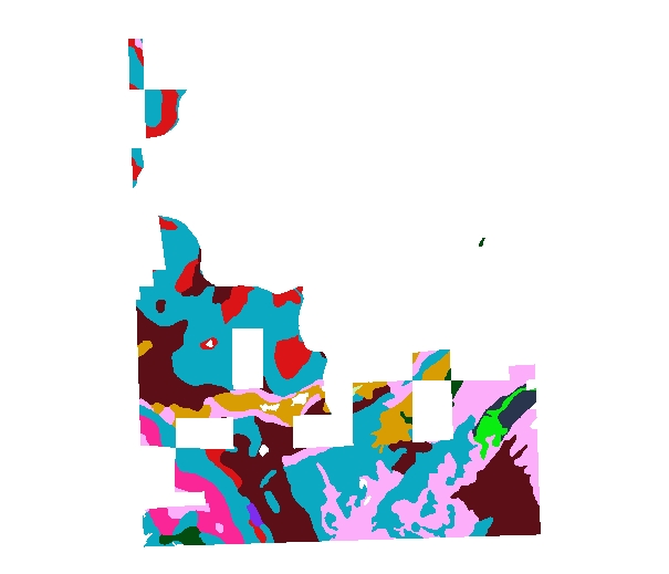
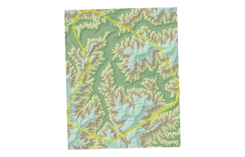
^ (SetNull2) In this exercise I used SETNULL to create a mask where non-Forest Service land and water bodies are set to NoData, and then used the mask to clip the Soil layer.

 

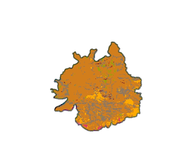
^ (Mosaic2)  In this exercise I assembled raster data for an area where a wildfire has occurred. I combined multiple input rasters into a single raster dataset through the process of mosaicking. As I worked through the steps, I saw how I can control raster processing.

I am now able to:

• Build Map Algebra expressions.
• Use Map Algebra operators.
• Use Map Algebra functions.
• Perform conditional processing.
• Work with NoData.

Module 4:  In this module, I learned about Spline and Inverse Distance Weighted (IDW), and was introduced to Kriging, a more powerful and complex interpolation method. The exercises allowed me to experiment with each of these interpolation methods.  

^  this exercise I used a sample point layer that represents elevation points at specific locations on and around the Shivwits Plateau in Arizona.

^

^ The goal in this exercise is to create a representative terrain surface from a recently collected sample point dataset. Elevation (in feet) was recorded at each location. A small portion of the Tallgrass Prairie National Preserve in the Flint Hills region of Kansas has been designated the special study area. 

I am now able to:

• List the basic principles of interpolation.
• Create surfaces using interpolation.
• Control sample points using interpolation.
• Use IDW, Spline, and Kriging.
• Explain what the interpolators covered have in common.

Module 5:  This module introduced me to ArcGIS® Spatial Analyst distance and density functions. Distance functions allow me to determine the nearest location of something or the least-cost path to a particular destination. Density functions, on the other hand, allow me to see the highest and the lowest concentrations of features in my data.

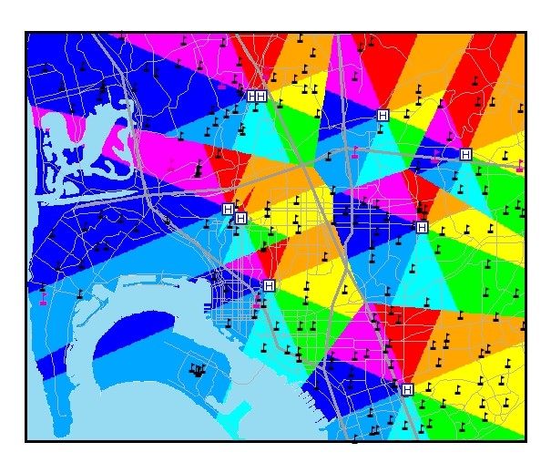
^ (Distance2) I built a model that uses the Euclidean Allocation tool to create surfaces of straight-line distance, direction, and allocation.  I used the distance surface to find the distance from the schools (locations on the surface) to the nearest hospitals (source). Next, I explored the direction and allocation surfaces. Finally, I used Map Algebra and the CON function to create a reverse direction surface of the Direction to the Hospital layer. This way, dispatchers can also help the pilots navigate back to the hospital.

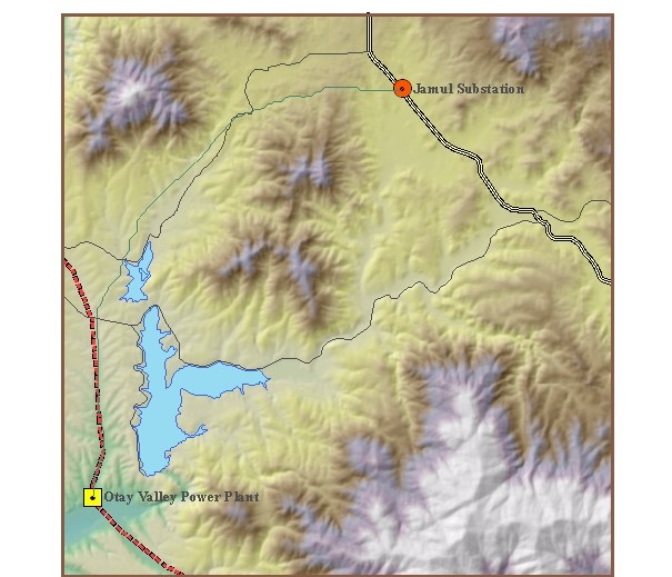
^  (FindPath2) The primary goal of this exercise is to find the least-cost path for a proposed power transmission line between a fictional power plant site (Otay Valley Power Plant) and substation (Jamul Substation) in Southern California. I balanced two important considerations: keeping construction costs down and minimizing risks to public safety.

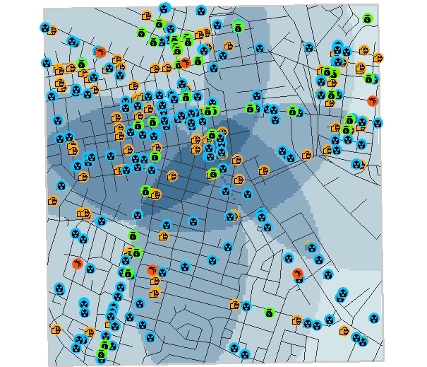
^ (CrimeStudy2)  In this exercise, I used the Density function to find patterns based on the location of six murders in a downtown study area. The density surface reveals underlying patterns that might not otherwise be evident.

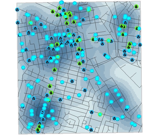
^ (Theft2)  In this exercise, I used the kernel option of the density function to find patterns based on the locations of burglary and grand theft in a downtown study area.

I am now able to:

• Create straight line distance, direction, and allocation surfaces.
• Create cost weighted distance, direction, and allocation surfaces.
• Perform a least-cost path analysis.
• Create density surfaces using the simple method.
• Create density surfaces using the kernel method.
• Create density surfaces using feature attributes.
 

Module 6: Spatial Analyst provides a set of statistical functions, which makes descriptive statistics part of the geographic analysis. For example, I compared the difference between values over time, cell-by-cell, construct a statistical filter to weed out unwanted values. Also assess past trends or the current status of features, or reveal the underlying structure of the data.

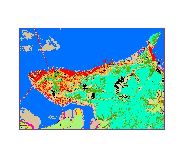
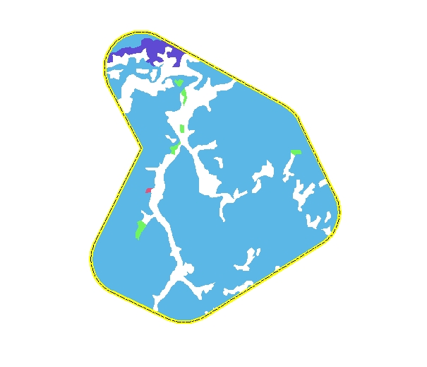
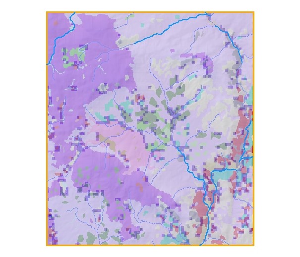
^ In this exercise, I used the Spatial Analyst Cell Statistics function to compare the 1989 to 1992 land cover data for a portion of the Columbia River Estuary, which is near where the Columbia River feeding into the Pacific Ocean. The land cover is classified based on vegetation groups, bare land, water, and developed areas.  

 ^ In this exercise, I  presented with a map of land cover types within a heavily forested area. Dominant vegetation types define the land cover. The patterns of different vegetation types are clearly distinguished, but the relationships between them are not.

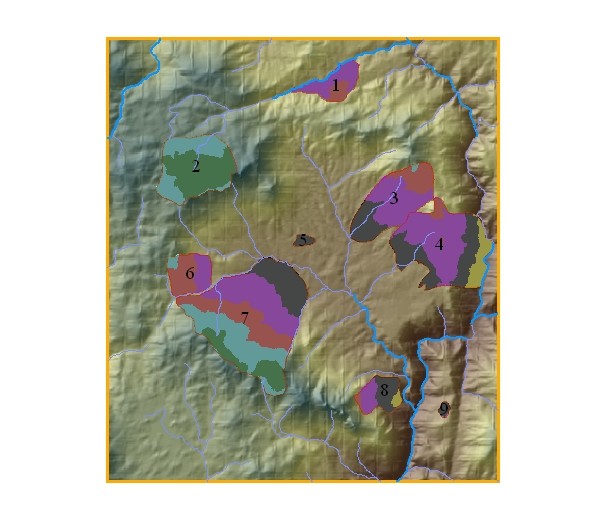
^ In this scenario, there have been a series of wild land fires in fairly rugged terrain, which is composed of heavily forested land. It would be interesting to know how many different types of trees and vegetation the fires affected, but it would also help to know where the variety occurred. 

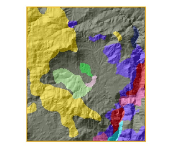
^ In this exercise, I  worked with a small quantity of vegetation data so I can see what happens as I progress through the functions. I removed detail in order to generalize some of the information in the map, but the way I removed it involves considering the majority values and dominant features. 

I am now able to:

• Recognize the types of statistical methods used in common by the three different statistical functions.
• Create new raster datasets using the Cell Statistics function.
• Create new raster datasets using the Neighborhood Statistics function.
• Analyze spatial data using the Zonal Statistics function.
• Generalize spatial data.
• Clean up NoData speckling in a raster dataset.

Top of Page