ESRI Virtual Campus: 3D Analyst
With ArcGIS 3D Analyst, I can add some real worldlike effects to my GIS data by displaying it in 3D. While a 3D representation of my data will often wow an audience, the extension also contains a powerful set of analytical tools. The following concepts introduced me to ArcGIS 3D Analyst and its four applications: ArcScene, ArcGlobe, ArcMap, and ArcCatalog.
Module 1: ArcGIS 3D Analyst; allows me to view, interact, and analyze data within a three-dimensional environment.

|
Mod1_complete.pdf Size : 154.125 Kb Type : pdf |
^
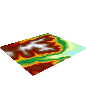
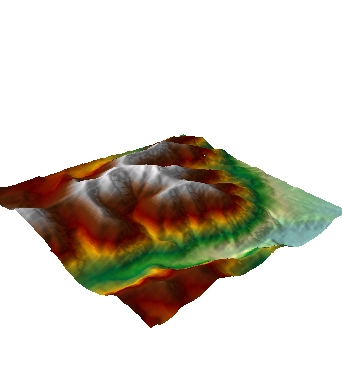
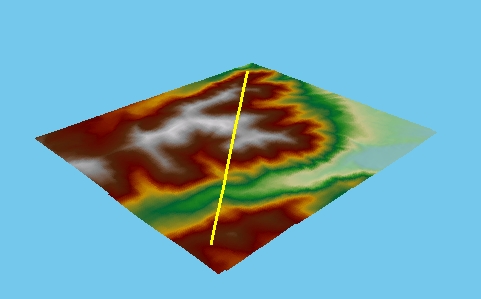
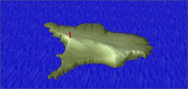
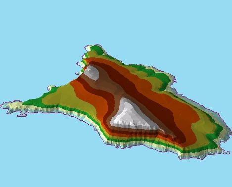
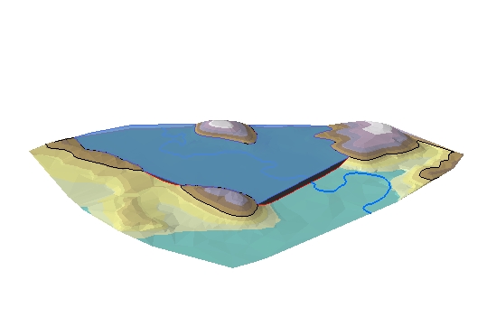
| In this exercise I previewed and explored 3D data for the Mt. Shavano area, which is located in south-central Colorado. |
^
| In this exercise I previewed and explored 3D data for the Mt. Shavano area in ArcScene. |
^ In this exercise I learned to navigate by using the Fly tool
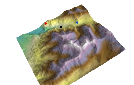
^ In this exercise, I used the Center on Target and Set Observer tools to look at a cabin at the base of Mt. Shavano from two different locations. I then used the Add Viewer tool to make a side-by-side comparison of the two perspectives.
^ In this exercise I used the view settings to control the x, y, and z coordinates of both observer and target exactly, as well as giving the exact line-of-sight distance between them. View settings also let me toggle between 2D and 3D views of the scene.
I am now able to:
- Describe the four components of ArcGIS 3D Analyst.
- Understand the purpose of z-values in 3D data.
- Distinguish between surfaces and feature data.
- Explain, in basic terms, how TINs and rasters model reality.
- Use the Navigate tool to pan, zoom, and rotate the 3D data.
- Define a 3D view perspective by setting target and observation points.
- Perform a fly-through of the 3D data.
Module 2: In this module, I learned how to control the appearance of the 3D environment then how to turn flat surfaces into landscapes, how to make buildings rise from the ground, how to drape aerial photographs over the landscape, and how to control light, shadow, and background color.
|
|
Mod2_complete.pdf Size : 152.994 Kb Type : pdf |
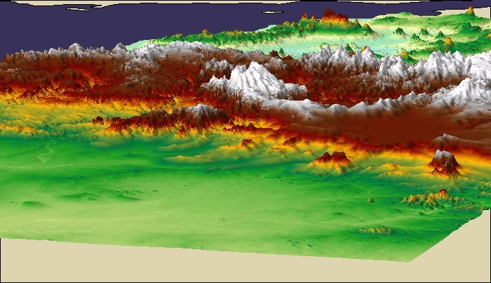
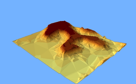
^ Vertical exaggeration lets me give a more dramatic appearance to terrain by emphasizing small changes in elevation.
^ In this exercise I learned that light and shade effects are an integral part of seeing things in 3D.
^ In this exercise I learned to improve navigation speed by changing a layer's refresh rate or by using a fast-drawing layer during navigation. I can also improve navigation speed by lowering the default raster resolution of raster layers. And I can improve raster display by increasing the raster resolution.
^
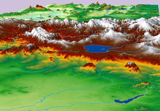
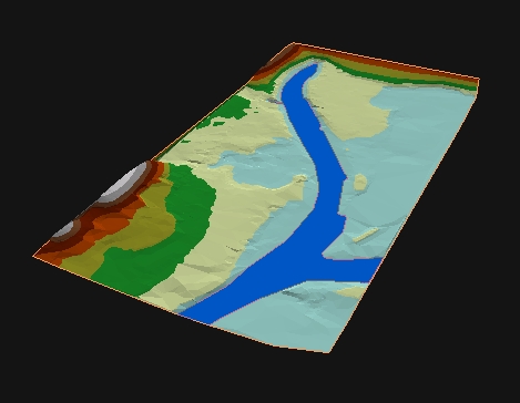
| All of the ordinary 2D spatial data can be displayed in 3D perspective, as long as I have a surface layer (raster or TIN) that has elevation values and the same extent as the 2D data. In this exercise, I added rivers and lakes to the Africa elevation surface |
^ Extrusion turns points into vertical lines, lines into walls, and polygons into solid blocks
I am now able to:
- Display flat data in 3D perspective.
- Make 3D features look bigger or smaller than they really are.
- Change the position of the "sun" to represent different times of day.
- Make features such as roads and rivers follow the contours of a 3D landscape.
- Drape air and satellite photos over terrain.
- Make features like buildings, walls, and poles rise from the ground to their actual height.
- Make 3D maps of attributes like income or population.
Module 3: In this module I am introduced to 3D symbols and how I can use them to render real-world objects. In 3D Analyst, the new 3D symbology includes true 3D symbols and realistic texture options.
|
|
mod3_fin.pdf Size : 154.284 Kb Type : pdf |
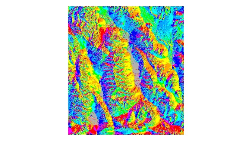
^ I learned to add or create a TIN in ArcScene and symbolize it by elevation. I can get different types of information from the TIN by rendering it in other ways. For example, I can draw my TIN to show slope or aspect
^ I continued types of customizations in this exercise by changing the classification ranges and enhancing the TIN with picture fills.
^ In this exercise I symbolized all edge types with a single symbol or with unique values and symbolized nodes with a single symbol, by elevation, or by tag values.
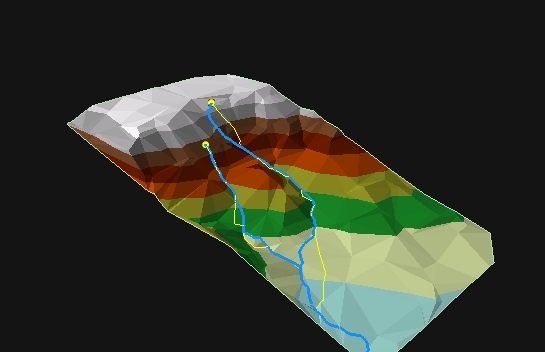
^ In this exercise, I found the steepest path from the headwaters (sources) of two different streams, then compared these to the actual stream locations.
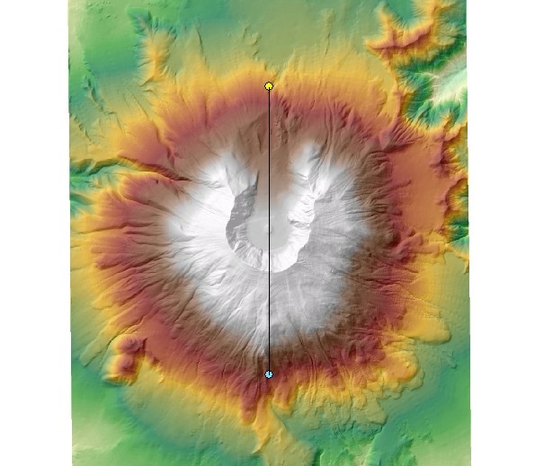
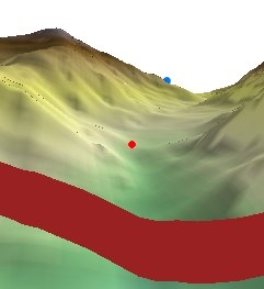
^ In this exercise, I created profile graphs that follow north-south and east-west lines of sight across the cone of Mount St. Helens.
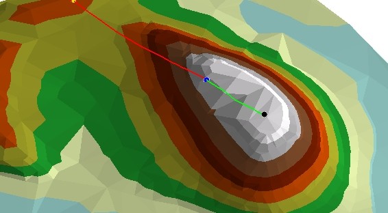
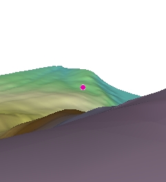
^ In this exercise, I had drawn a line of sight between two points of a proposed site for wildlife observation and a badger den.
^ This exercise introduced me to several ways to run 3D Analyst geoprocessing tools such as slope and aspect.
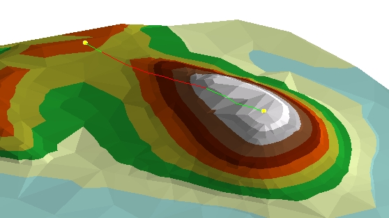
^ In this exercise I created a line of sight between the same observer and target point, but this time I used the Line of Sight geoprocessing tool, which works a little differently.
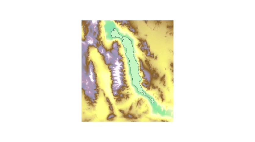
^ In this exercise, I calculated the area and volume of a proposed lake named Muddy Puddle. The desired elevation of the water table is 1,114 feet above sea level. The lake level is expected to fluctuate seasonally between 1,100 and 1,114 feet.
I am now able to:
- Use renderers to change the way a TIN is drawn.
- Change the data classification used to symbolize a TIN.
- Add more realistic symbolization to TIN data using picture fills.
- Use 3D symbols and textures to render points, lines and polygons.
- Set geoprocessing environment settings.
- Run 3D Analyst tools from their dialog box, the command line, or from within a model.
- Find steepest path lines on a surface.
- Create profile graphs for lines drawn on surfaces.
- Determine if a target is visible from an observer location.
- Find out which portions of a line of sight are visible.
- Calculate area and volume statistics.
Module 4: In this module, I will create TIN surfaces from feature layers and 3D features by digitizing on a TIN or raster surface. I will also convert data from one format to another. 3D Analyst can convert rasters to TINs and TINs to rasters.
|
|
Mod4_fin.pdf Size : 153.355 Kb Type : pdf |
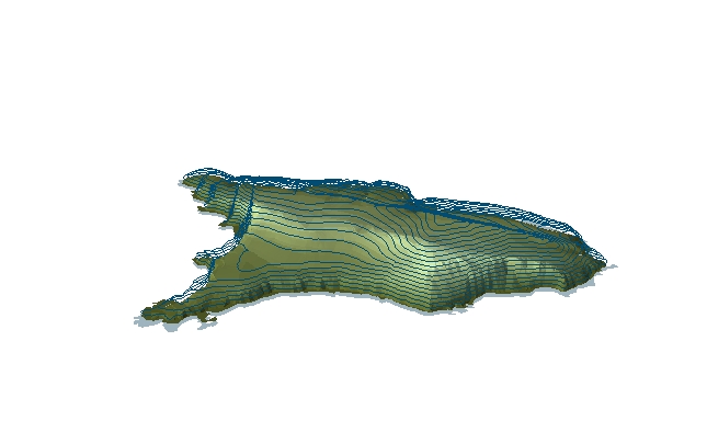
^ In this exercise, I used the geoprocessing tools in ArcToolbox to create and populate a TIN with features from elevation contours of Santa Barbara Island. Then I clipped the TIN to the boundary of the shoreline.
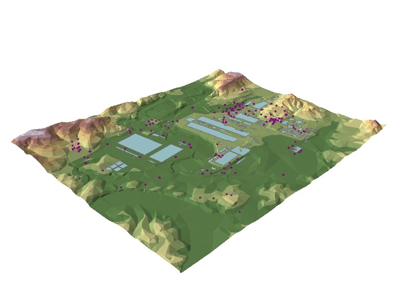
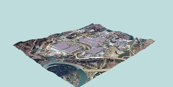
^ In this exercise, I converted 2D layers of buildings and wells to 3D. I worked with the Oak Ridge, Tennessee data.
^ In this exercise, I incorporated all the layers at once, completing the TIN in one stroke.
I am now be able to:
- Create a TIN surface.
- Modify an existing TIN.
- Convert 2D features to 3D.
- Create new 3D features.
- Convert rasters to TINs and TINs to rasters.
- Convert TINs and rasters to feature layers.
- Create and display terrains.
- Use terrains in surface analysis operations.
- Convert terrains to rasters.
Module 5: Calculating Raster Surfaces.
In this module, I modified rasters for new information. This new information is usually provided in the form of another raster.
|
|
Mod5_fin.pdf Size : 153.714 Kb Type : pdf |
^ In this exercise, I created surface analysis rasters of hillshade and aspect.
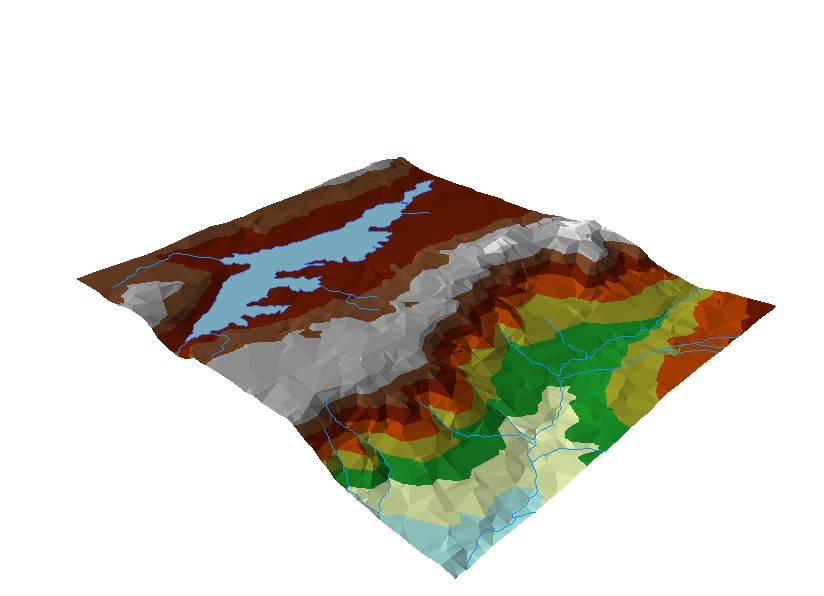
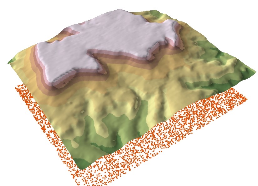
^ In this exercise, I reclassified a raster to find areas that have elevation values below sea level. I then converted the reclassified raster to a feature layer, creating a polygon shapefile of the floor of Death Valley.
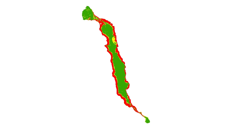
^ In this exercise, I calculated slope for the floor of Death Valley—the area at or below sea level that I isolated in the previous exercise.
I am now able to:
- Calculate slope, aspect, and hillshade rasters from elevation rasters.
- Calculate viewshed rasters for one or many observer locations.
- Reclassify a raster.
- Set raster analysis options, such as working directory, mask, and analysis extent.
Module 6: Interpolating Raster Surfaces
In this module, I learned some of the theory of spatial interpolation. Spatial interpolation is the process of estimating unknown geographic values on the basis of known values and what makes it possible to create realistic surfaces from a limited number of sample points.
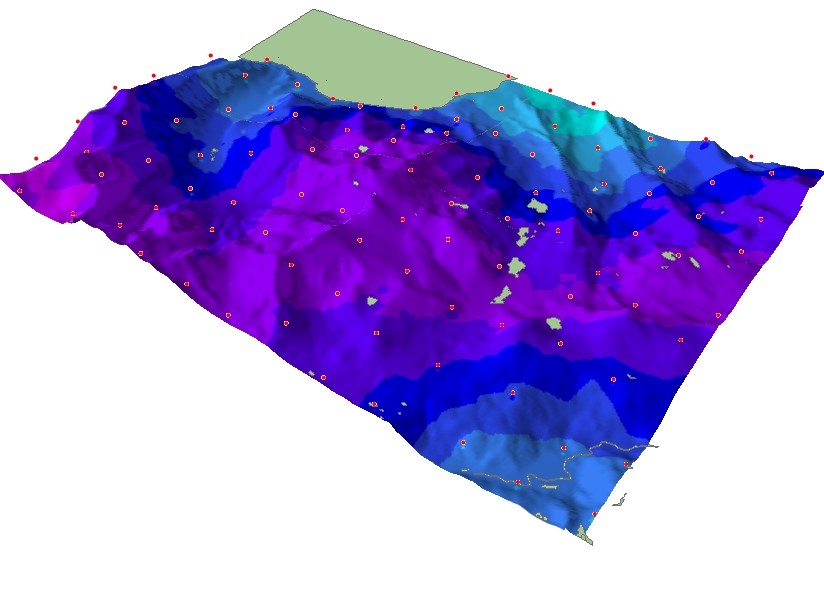
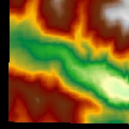
^ I Used IDW to interpolate three alternative surfaces of snow depth: one with default parameters, one with a lower power setting, and one with a fixed search radius. Before interpolating the surfaces, I then used a mask to exclude Lake Tahoe from the analysis.

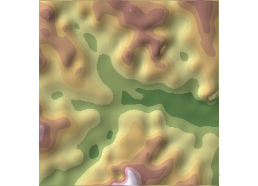
^ this exercise, I was provided with a sample point layer that represents drill holes used to penetrate the top of a subsurface limestone formation. In this case, exploratory drilling has indicated the presence of oil, and the depths of the drill holes will be used to model the bending of the limestone surface.

|
Tallgrass2_dl_6_3.jpg Size : 142.507 Kb Type : jpg |
^ One advantage of the Spline interpolator is that it can make estimates outside of the range of input sample points. There are two types of spline interpolators. The regularized spline creates a more elastic surface. The tension spline creates a stiffer surface.
^ In this exercise, I used the Natural Neighbor interpolation method to create an elevation surface from sample points around the Shivwits Plateau in Arizona.
I am now be able to:
- Describe the principles underlying spatial interpolation.
- Create raster surfaces using the Inverse Distance Weighted method.
- Create raster surfaces using the Spline method.
- Create raster surfaces using the Natural Neighbors method.
- Understand why the Kriging method is unique
Module 7: Introduction to ArcGlobe:
This module introduced me to ArcGlobe. Available with ArcGIS 3D Analyst, ArcGlobe allows interactive 3D visualization and analysis of spatially referenced data on a 3D globe surface. By interacting with the data in ArcGlobe, I can explore the entire planet or focus on local areas. In ArcGlobe I can work seamlessly with terabytes of data without having to preprocess it.