Module 1: Sizing Up the Earth - This module discusses the earth's shape, size, and spherical coordinate system, and presents the basics of map projections. With the complestion of this module, I am now able to:

^ In this exercise, I learned how projections are not a perfect spheroid. The earth's surface is not perfectly symmetrical, so the semi-major and semi-minor axes that fit one geographical region do not necessarily fit another one. Many different spheroids are used throughout the world to account for these deviations. WGS 1984, International 1924, and Clarke 1866 are shown in the image above from ArcMap. As you can see, the areas around the body of water show that there are distinctions amongst the projections. The map is showing the New York City area and Long Island.
Module 2: Flattening the Earth - In this module I learned about Map projections and how they represent the round earth on a flat medium such as a sheet of paper or a computer screen. Conceptually, many projections are made on a surface that can be flattened without distortion such as a plane, a cylinder, or a cone. Many of the map projections used today were invented during and after the Renaissance.
With the completion of this module, I am now able to:

^ In this exercise, I looked at several world map projections and saw how they distort such spatial properties as shape, area, and distance.
The map display shows the world in the Plate Carrée map projection. There are four data layers. The Ellipses are circular near the equator and become bean-shaped towards the poles. I learned that not all map projections preserve the same properties.
Module 3: Understanding Aspect and Perspective - In this module I learned about aspect, which is the orientation of a projection with respect to the earth's axis. A way to look at it is; if the projection surface is a plane, this plane might touch the globe at the north pole, or at a point on the equator, or somewhere in between. Each of these variations gives the projection a different appearance and different use. I also explored perspective. A perspective projection is one that can be constructed with geometry. A nonperspective projection is one that uses more elaborate math.
After completing this module, I am now able to:

^ In this exercise, I looked at a world Mercator projection in its equatorial, transverse, and oblique aspects. The choice of aspect for a cylindrical projection largely depends on the shape of the area of interest. For areas oriented east to west, an equatorial aspect is best. For areas oriented north to south, a transverse aspect is best. And for areas that run slantwise (like the Hawaiian or Aleutian islands) an oblique aspect is best.

^ In this exercise, I looked at an Azimuthal Equidistant projection in its normal, transverse, and oblique aspects. The valuable property of this projection is that it preserves true distance and true direction from a single point to any location on the map. The choice of aspect is determined by the point of interest. This projection is probably most often used for polar maps, but can be used for a map centered on any important point. Since it has no east–west or north–south bias, it can also be used to map landmasses, like Asia, that spread fairly equally in all directions. Any line drawn from the center of the projection follows a great circle, the Azimuthal Equidistant projection is good for showing shortest-distance paths, like those followed by radio waves. Since it preserves true distance, it is also good for plotting ranges, such as the range of an airplane from a base, or the decay rates of light or noise from a source.

^ In this exercise, I looked at three perspective planar projections, the Gnomonic, the Stereographic, and the Orthographic. None of these three can project the entire world (half the coordinates, more or less). In the case of the Gnomonic projection, the angle between the wires and the surface is such that some coordinates miss the map surface entirely and slide off into eternity.
Module 4: Examine perspective - In this module, I worked with a number of common projections and learn about the spatial properties they distort. I also learned how to set up a projection to minimize distortion in the area of interest. Every map has some distortion. In a map of a small area, distortion may be negligible; in a map of a large area, it will be significant. So, Choosing a map projection means choosing a distortion. Sometimes it's good to stay faithful to one spatial property and leave another out. So when it comes to making a map, not only is it important to choose a projection, it's also good to tailor it to the specific part of the world of interest. Having as little of distortion as possible in the area of interest is important, and allowing more distortion in places that may not be shown on the final map at all can be accecptable.
In the first exercise, I looked at distortion diagrams for the Mercator, Lambert Azimuthal Equal Area, and Equidistant Conic projections in the Index provided with the training course. http://training.esri.com/Courses/MapProjections/M4/map_projection_summary_index28214.cfm

^ In this exercise, I worked with the Equidistant Conic and Albers Equal Area Conic projections. Taking North America as the area of interest first, then looked at how the property of shape is affected by the choice of tangent and secant lines. I also worked with a Polyconic projection of the world and looked at its overall effect on shape.


^ In this exercise, I chose projections for three maps related to the theme of the Spanish conquest of Mexico. The first map is a general reference map, orienting map readers to the geographic relationship between Mexico, Cuba, and the islands of the Caribbean with the Azimuthal Equidistant projection. The second map's purpose is area comparison that shows how much land in Mesoamerica was controlled by the Aztecs. I chose an equal area projection called Albers equal area conic. The third map's purpose is to represent Cortes's route, not the distance he traveled, but the configuration. This requires, for the sea voyage, that the shape of the coastline be true; for the march inland, it means accurately depicting the twists and turns along the way. To represent the shapes of features accurately, I used a conformal projection called Lambert Conformal Conic.
Module 5: Geographic and Planar Coordinate Systems - We have the means to describe a location as so many squares to the left, so many to the right, so many up, or so many down, and at last we have its number. (Adapted from Watts, 1966). Coordinate systems identify locations by making measurements on a framework of intersecting lines that resemble a net. On a map, the lines are straight and the measurements are made in terms of distance. On a round surface (the earth) the lines become circles and the measurements are made in terms of angle. The goal of this module is to define what coordinate systems are and how they work.
With the completion of this module, I am now able to:
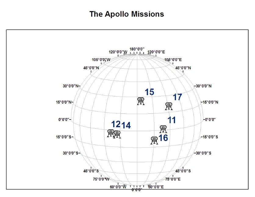
^ In this exercise, I started from scratch and defined my own geographic coordinate system. I used a text file with point data from the moon in lunar latitude/longitude coordinates. ArcMap™ doesn't have a GCS for the moon, so I defined one. Then I added lunar layers and took some measurements. In the end, I compared some earthly measurements to prove that indeed I was working with a sphere that is aproximately the size of the moon.
Module 6: Introduction to Datums - Starting values on a map projection are known as a datum. In this module, I learned about the elements that compose a datum and witnessed how one person's latitude-longitude coordinates can be matched up with another's in a process called datum transformation. Since this is a recurring problem for GIS users, the exercises in this module are devoted to helping the datasets complexity that have different geographic coordinates.
With the completion of this module, I am now able to:
In the first exercise, I worked with two datasets that have no coordinate system information. I then determined their coordinate system with the help of ArcCatalog and other useful information, then used ArcGIS to add this information permanently to each data source.

^ In this exercise, I learned how ArcMap applies its default datum transformations and how to change these settings. I changed the data frame's GCS from NAD27 to NAD83. This lets it apply the very accurate NADCON transformation to align the streets and parcels. It also lets the transform between WGS84 and NAD83 (instead of between WGS84 and NAD27) to align the parcels and hydrants. This is an advantage because WGS84 and NAD83 are both earth-centered datums with similar specifications; consequently, this transformation is more accurate.